The lecture material for this lecture was as follows:
Hidden Markov Model (HMM) is a special kind of Markov Model (MM) which is based on probability theory. The first video lecture is a repetition of probability theory.

Lecture 2 and 3 is about Bayes nets utilizing the Bayes rule. From machine learning I we remember the Naive Bayes (Naive Bayes Belief Network) where we assumed all random variables (our features) were independent. P(A|B) = P(A).
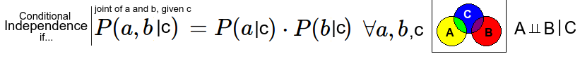
In Bayes nets (BN) we don't assume independence, but we assume conditional independence. Lets say we have 3 observations A, B and C. A leads to C and C leads to B. We now assume that A and B are conditional independent when C is known. In the video A is fire, C is smoke and B is smoke detector triggering.
Bayes net will have a topology (directed acyclic graph) and a conditional probability table for each variable. We only assume that the probability of a variable is only dependent on the parent of the variable. The parents are other variables pointing directly at this variable in the graph. We can build these graphs based on believed causation, but causation is not an assumption made in Bayes nets.
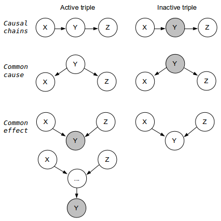
Lecture 3 explains the different types of active triples in order to determine whether independence can be guaranteed or "not guaranteed"
We can guarantee independence of two variables if all paths are inactive. A path is inactive if one or more triples are inactive.
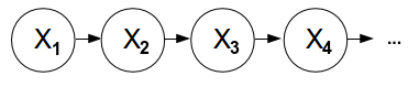
The fourth lecture is the one about Hidden Markov Models, and it explains HMM are used for "reasoning about sequences of observations". Typical examples are speech recognition, localization and medical monitoring. A Markov model is chain-structured Bayesian Network (BN). We then assume previous and future states are conditional independent given the current state. The conditional probability table is constant for all states.
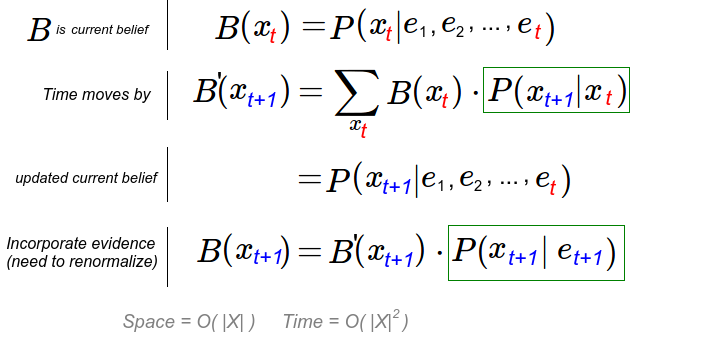
The mini-forward algorithm will give you the stationary distribution, and means that the influence of the first observation is forgotten over time. Web link analysis and Gibson sampling were two examples of use of Markov models, but in order for them to be more useful we need to feed it with observations so to update the beliefs based on evidence.
A Hidden Markov Model is such a model where we are not able to measure the wanted effect directly, but we can do it indirectly, like this:
We need
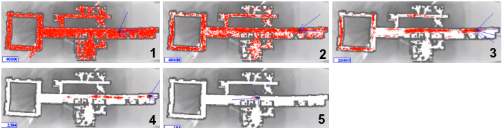
Solutions to speed this up include using particle filtering
https://www.youtube.com/watch?v=Qh2hFKHOwPU
- [1] Lecture12: Probability
- [2] Lecture 13: Bayes' Nets 1
- [3] Lecture 14: Bayes Nets II Conditional Independence
- [4] Lecture 18: Hidden Markow Models
Hidden Markov Model (HMM) is a special kind of Markov Model (MM) which is based on probability theory. The first video lecture is a repetition of probability theory.
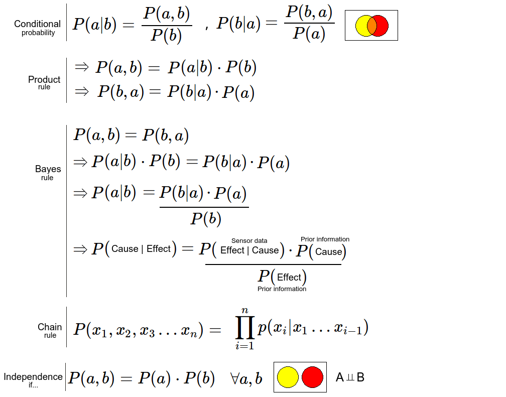
- Random variables: A random variable is a collection of possible outcomes, typically notated with uppercase letters. It can have many outcomes where each of the outcomes must have a probability of 0 or greater and the sum of them all must be 1 or 100%.
- Joint and marginal distributions: P(A, B) is the joint of P(A) and P(B). Finding the marginal is determining P(A) and P(B) from P(A, B). Also note that P(A, B) is the same as P(B, A). The order is not relevant for joints.
- Conditional distributions: P(A | B) is the "probability of A given B". This is when we know the outcome of B, and this changes the probability of A if they are dependent.
- Normalization trick: An easier way to calculate conditional probability by skipping the division step until last and then normalize the relevant values.
- Product rule: Derived from the definition of conditional probability.
- Chain rule: Also derived from conditional probability
- Bayes rule and inference: Since joint probabilities are independent of order, we can substitute and express probability of A given B as B given A.
- Independence: If A and B are independent, then we can simplify the product rule. Do not assume this is the case unless it holds for all A and B.
Lecture 2 and 3 is about Bayes nets utilizing the Bayes rule. From machine learning I we remember the Naive Bayes (Naive Bayes Belief Network) where we assumed all random variables (our features) were independent. P(A|B) = P(A).
In Bayes nets (BN) we don't assume independence, but we assume conditional independence. Lets say we have 3 observations A, B and C. A leads to C and C leads to B. We now assume that A and B are conditional independent when C is known. In the video A is fire, C is smoke and B is smoke detector triggering.
Bayes net will have a topology (directed acyclic graph) and a conditional probability table for each variable. We only assume that the probability of a variable is only dependent on the parent of the variable. The parents are other variables pointing directly at this variable in the graph. We can build these graphs based on believed causation, but causation is not an assumption made in Bayes nets.
Lecture 3 explains the different types of active triples in order to determine whether independence can be guaranteed or "not guaranteed"
We can guarantee independence of two variables if all paths are inactive. A path is inactive if one or more triples are inactive.
The fourth lecture is the one about Hidden Markov Models, and it explains HMM are used for "reasoning about sequences of observations". Typical examples are speech recognition, localization and medical monitoring. A Markov model is chain-structured Bayesian Network (BN). We then assume previous and future states are conditional independent given the current state. The conditional probability table is constant for all states.
The mini-forward algorithm will give you the stationary distribution, and means that the influence of the first observation is forgotten over time. Web link analysis and Gibson sampling were two examples of use of Markov models, but in order for them to be more useful we need to feed it with observations so to update the beliefs based on evidence.
A Hidden Markov Model is such a model where we are not able to measure the wanted effect directly, but we can do it indirectly, like this:
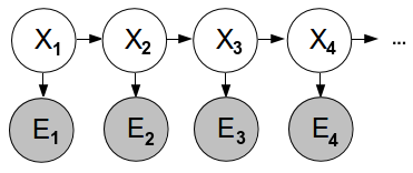
We need
- An initial distribution for X: P(first X)
- Transition from X to next X: P(X|previous X)
- Emission, probability of measurement being correct: P(X|E)
Solutions to speed this up include using particle filtering
https://www.youtube.com/watch?v=Qh2hFKHOwPU