Artificial Neural Networks are Machine Learning methods inspired by how the biological brain, the most intelligent entity known in nature, in order to make machines perform intelligent behavior. ANN was very popular in the 80's, lost a lot of ground during the 90's, and has come back quite strong recently. One of the reasons why they are so popular is that they consists of very simple, highly interconnected building blocks, and even though one might think the brain would have to need a whole lot of different algorithms in order to learn all we (or any advanced animal) is capable of, rewiring experiments has shown that the location receiving visual, auditory, touch or any other signal with a pattern will learn to make use of it, as if there is only a single (simple) algorithm responsible for learning.

(The perceptron)
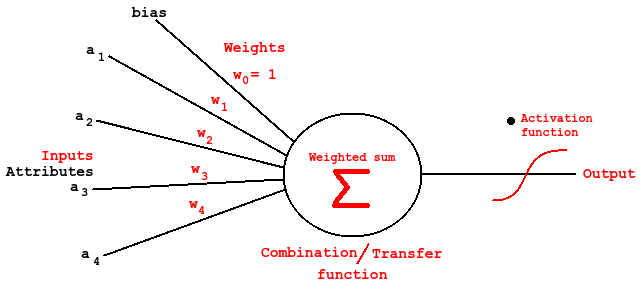
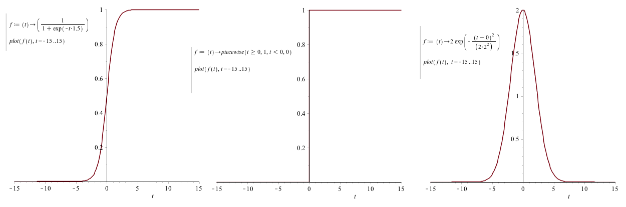
The most basic building block in the brain is the neuron, a cell (nucleus) capable of communication with neighbor cells via input (dendrite) and output (axon) wires. Typically 10⁴. The axons can be more than a meter long in order to control limbs far away. The brain keeps rewiring it's neurons and the connectivity will be enforced or weaken depending on how useful they are. This is simulated by weighted inputs in ANN, and usually a summed product of inputs / features (combination function) are feed to an activation function before it's output. The activation function can be things like step function, sign activation, sigmoid, Gaussian and even linear. (See This book at Google books for reference)
The simplest ANN would be only using one neuron (single). By adding more layers, we usually call the layer receiving the attributes the “input layer”, and the neurons at the end are the “output layer”. There can be one or multiple neurons in these layers. In a multi classification problem one typically have one output “node” for every classification. As an extension, called multi layered, there are one or more “hidden” layers in between the input and output layers. They are called hidden because their output is not directly observable. The main idea of multiple layers is that the power of neural networks comes from incremental pattern recognition where each layer is able to “understand” more abstract (non linear) patterns (like how the current understanding of how the neocortex is functioning)
ANN can be feed forward, meaning computation is performed from input to output (in parallel in the brain, and usually simulated on computers). This is what is most like the biological behavior, although we know there is some feedback to cells via the dendrites.
One way to make the ANN learn is to back propagate the error (difference between known class/value) and adjust the weights up or down accordingly via gradient descent search. The weights are initialized at random.
Some interesting videos
Video: Neural networks
Video: Evolution of simple organisms with neural networks
The Next Generation of Neural Networks
Video lecture: ANN by Andrew Hg (Stanford)
8.1: Non linear hypothesis
8.2: Neurons and the brain
8.3: Model representation I
8.4: Model representation II
8.5: Examples and intuition I
8.6: Examples and intuition II
8.7: Multi-class classification
8.8: Autonomous driving example
9.1: Cost function
9.2: Back propagation
9.3: Back propagation intuition
9.4: Gradient checking
9.5: Random initialization
9.6: Examples and intuition II
9.7: Putting it together
9.8: Autonomous driving example
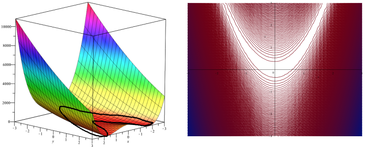
During the exercise we did gradient descent on this function:
(The perceptron)
The most basic building block in the brain is the neuron, a cell (nucleus) capable of communication with neighbor cells via input (dendrite) and output (axon) wires. Typically 10⁴. The axons can be more than a meter long in order to control limbs far away. The brain keeps rewiring it's neurons and the connectivity will be enforced or weaken depending on how useful they are. This is simulated by weighted inputs in ANN, and usually a summed product of inputs / features (combination function) are feed to an activation function before it's output. The activation function can be things like step function, sign activation, sigmoid, Gaussian and even linear. (See This book at Google books for reference)
The simplest ANN would be only using one neuron (single). By adding more layers, we usually call the layer receiving the attributes the “input layer”, and the neurons at the end are the “output layer”. There can be one or multiple neurons in these layers. In a multi classification problem one typically have one output “node” for every classification. As an extension, called multi layered, there are one or more “hidden” layers in between the input and output layers. They are called hidden because their output is not directly observable. The main idea of multiple layers is that the power of neural networks comes from incremental pattern recognition where each layer is able to “understand” more abstract (non linear) patterns (like how the current understanding of how the neocortex is functioning)
ANN can be feed forward, meaning computation is performed from input to output (in parallel in the brain, and usually simulated on computers). This is what is most like the biological behavior, although we know there is some feedback to cells via the dendrites.
One way to make the ANN learn is to back propagate the error (difference between known class/value) and adjust the weights up or down accordingly via gradient descent search. The weights are initialized at random.
Some interesting videos
Video: Neural networks
Video: Evolution of simple organisms with neural networks
The Next Generation of Neural Networks
Video lecture: ANN by Andrew Hg (Stanford)
8.1: Non linear hypothesis
8.2: Neurons and the brain
8.3: Model representation I
8.4: Model representation II
8.5: Examples and intuition I
8.6: Examples and intuition II
8.7: Multi-class classification
8.8: Autonomous driving example
9.1: Cost function
9.2: Back propagation
9.3: Back propagation intuition
9.4: Gradient checking
9.5: Random initialization
9.6: Examples and intuition II
9.7: Putting it together
9.8: Autonomous driving example
During the exercise we did gradient descent on this function:
import math
import os

os.system("clear")

step_size = 0.00001
start_point = [0.9, 1.1]
iterations_max = 1000
climb = -1  # 1: up, -1: down


def f(x, y):
	x = float(x)
	y = float(y)
	return math.pow((1 - x), 2) + 75 * math.pow(y - math.pow(x, 2), 2)

pos = start_point
print("Step size: %s, max iterations: %s, %s") % (step_size, iterations_max, ("climbing") if climb > 0 else "descending")
print("Starting point: (%s, %s)") % (round(pos[0], 3), round(pos[1], 3))


def gradient_search(pos, iterations_max, step_size, climb):
	old_pos = pos[:]
	best_pos = pos[:]
	step = step_size
	for i in range(0, iterations_max):
		# Check each variable: decide direction to walk
		current_value = f(pos[0], pos[1])
		diff_x = f(pos[0] + step, pos[1])
		diff_y = f(pos[0], pos[1] + step)

		total_diff = diff_x + diff_y
		rel_x = (diff_x / total_diff) * step * climb
		rel_y = (diff_y / total_diff) * step * climb

		#print("%s at round %s") % (round(current_value), i + 1)
		if ((-1 * climb) * current_value) < f(best_pos[0], best_pos[1]):
			best_pos = pos[:]

		if current_value < diff_x:
			pos[0] += rel_x
		else:
			pos[0] -= rel_x

		if current_value < diff_y:
			pos[1] += rel_y
		else:
			pos[1] -= rel_y

		new_value = f(pos[0], pos[1])

		if (-1 * climb) * new_value > f(old_pos[0], old_pos[1]):
			pos = old_pos[:]
			step = step_size
		else:
			step += step_size
		#print step

		old_pos = pos[:]

	return [best_pos, i + 1]


pos = gradient_search(pos, iterations_max, step_size, climb)

print("Final (local) optimum: (%s, %s) in %s tries (value: %s)\n") % (round(pos[0][0], 3), round(pos[0][1], 3), pos[1], f(pos[0][0], pos[0][1]))