As a short recap, we continue in the model of pattern recognition. The last lecture was about searching as a part of learning, and the first lecture was about the model in itself and the first step preprocessing. (The 2nd was benchmarking). Now we look at what's between preprocessing and the learning phase.
The main difference between feature selection and extraction is whether we do any transformations on the original attributes (that might already be manipulated in the preprocessing step) or not. Feature selection is basically ranking the attributes based on how "useful" they are, and then go for the top most useful. The reason for removing redundant attributes is that they increase the complexity "search space" / "hypothesis space" to look trough in order to find optimal learning rules / knowledge.
In feature extraction we either transform the whole attribute space to another space (like principle component analysis (PCA)) or do some kind of combining of attributes to form new ones. Like attribute 1 multiplied (*), divided by (/), XORed, ORed, ANDed etc... with attribute 2
Heuristic search (in this setting for optimal (combinations) of attributes can also be heuristic or brute force. Being heuristic means we realize there is no way to find the perfect solution, but we are going to mix in some randomness and use information about current best solution to choose other things to consider. With a heuristic method we only need a "good enough" solution.
The goal is simply to reduce the amount of work of the learning algorithm / classifier. Both during learning and during classification/regression.
Methods are divided in Wrapper models and Filter models. Wrappers are simply using a machine learning algorithm (like kNN, SVM, ANN) as a black box, try different combinations of raw features and see what features gives the best result. This is very slow as the "black box" we are using is very complex in it self. Still, by doing this we "fit" the attributes nicely to the chosen algorithm. To speed it up, we introduce so called Filter models. They again are divided in ranking and subset selection. The first is the most basic and fastest. We calculate some impurity measure of each attribute independently of each other and rank them. When we compare the impurity of one attribute with another one, the difference is said to be a quality measure. (is this true?). In subset selection we try combinations of attributes and for example if the combination is better at predicting (correlated with) the classification label.
Impurity (myopic) measures for ranking
Methods for subset selection
In order to get the best from both world we can first reduce the number of attributes by filter models and then apply wrapper model on the rest. This is called Embedded model
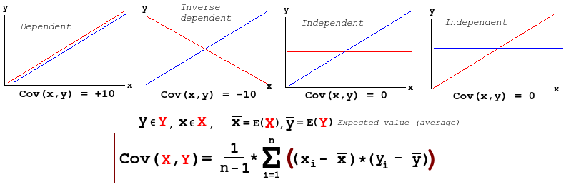
Covariance (used in PCA)

PCA and LDA
Video lecture on youtube
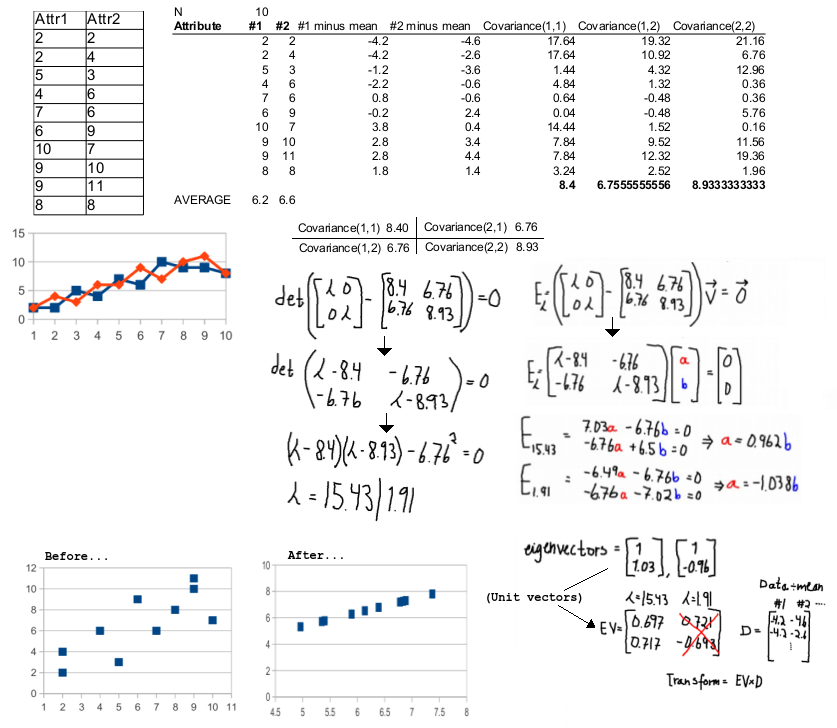
PCA (Principal Component Analysis) is an algorithm for reducing the number of dimensions in samples. The idea is to project higher dimensions down, and we want to project so that the information loss is minimum, we we achieve that by projecting where the variance is the highest. First data is normalized by subtracting attribute mean and spread, then we calculate the average covariance for every combination of attributes and put them in a matrix. We then find the eigenvalues and eigenvectors for this matrix. We can then remove the eigenvectors with the lowest eigenvalues. See this video for how to calculate eigenvalues and vectors.
The method is nicely described by Andrew Hg in this video: Lecture 14 | Machine Learning (Stanford) (05:22 and 38:44 are illustrations). There is no classification information available, so this method is good for verification.
A try at the exercise is given here:
Matrix calculator is a great tool.
LDA (Linear Discriminant Analysis) is also trying to reduce the number of dimensions, but at the same time it tries to keep class separation by utilizing known classification information on the samples. Since projecting in the direction of highest variance might divide / project the samples in a way "destroying" the possibility to later classify, we want to choose a "direction" that maximizes both (binary) class separation and variance. This is done by rotating the axis. This method is good for identification (claim)
During the exercises we discussed why we measure attribute quality. We calculated entropy, minimum description length on a string, performed PCA, did shannon-fano coding and calculated gini-index and classification error.
The main difference between feature selection and extraction is whether we do any transformations on the original attributes (that might already be manipulated in the preprocessing step) or not. Feature selection is basically ranking the attributes based on how "useful" they are, and then go for the top most useful. The reason for removing redundant attributes is that they increase the complexity "search space" / "hypothesis space" to look trough in order to find optimal learning rules / knowledge.
In feature extraction we either transform the whole attribute space to another space (like principle component analysis (PCA)) or do some kind of combining of attributes to form new ones. Like attribute 1 multiplied (*), divided by (/), XORed, ORed, ANDed etc... with attribute 2
Heuristic search (in this setting for optimal (combinations) of attributes can also be heuristic or brute force. Being heuristic means we realize there is no way to find the perfect solution, but we are going to mix in some randomness and use information about current best solution to choose other things to consider. With a heuristic method we only need a "good enough" solution.
The goal is simply to reduce the amount of work of the learning algorithm / classifier. Both during learning and during classification/regression.
Methods are divided in Wrapper models and Filter models. Wrappers are simply using a machine learning algorithm (like kNN, SVM, ANN) as a black box, try different combinations of raw features and see what features gives the best result. This is very slow as the "black box" we are using is very complex in it self. Still, by doing this we "fit" the attributes nicely to the chosen algorithm. To speed it up, we introduce so called Filter models. They again are divided in ranking and subset selection. The first is the most basic and fastest. We calculate some impurity measure of each attribute independently of each other and rank them. When we compare the impurity of one attribute with another one, the difference is said to be a quality measure. (is this true?). In subset selection we try combinations of attributes and for example if the combination is better at predicting (correlated with) the classification label.
Impurity (myopic) measures for ranking
- Entropy
- Information Gain
- Classification error
- Distance measure
- Minimum Description Length (Like encoding information with the fewest possible bits - shannon-fano and morse coding)
- J-measure
- Gini-index
Methods for subset selection
- Principle Component Analysis (PCA) (Actually unsupervised learning?)
- Linear Discriminant Analysis (LDA)
- Relevance
- Redundancy
- mRMR (mutual information)
- ReleifF
In order to get the best from both world we can first reduce the number of attributes by filter models and then apply wrapper model on the rest. This is called Embedded model
Covariance (used in PCA)
PCA and LDA
Video lecture on youtube
PCA (Principal Component Analysis) is an algorithm for reducing the number of dimensions in samples. The idea is to project higher dimensions down, and we want to project so that the information loss is minimum, we we achieve that by projecting where the variance is the highest. First data is normalized by subtracting attribute mean and spread, then we calculate the average covariance for every combination of attributes and put them in a matrix. We then find the eigenvalues and eigenvectors for this matrix. We can then remove the eigenvectors with the lowest eigenvalues. See this video for how to calculate eigenvalues and vectors.
The method is nicely described by Andrew Hg in this video: Lecture 14 | Machine Learning (Stanford) (05:22 and 38:44 are illustrations). There is no classification information available, so this method is good for verification.
A try at the exercise is given here:
Matrix calculator is a great tool.
LDA (Linear Discriminant Analysis) is also trying to reduce the number of dimensions, but at the same time it tries to keep class separation by utilizing known classification information on the samples. Since projecting in the direction of highest variance might divide / project the samples in a way "destroying" the possibility to later classify, we want to choose a "direction" that maximizes both (binary) class separation and variance. This is done by rotating the axis. This method is good for identification (claim)
During the exercises we discussed why we measure attribute quality. We calculated entropy, minimum description length on a string, performed PCA, did shannon-fano coding and calculated gini-index and classification error.
import math

information = "ababcaaabbbbcacbddartyeababafa"
num = len(information)
s = [
		{'char': 'a', 'freq': 11},
		{'char': 'b', 'freq': 9},
		{'char': 'c', 'freq': 3},
		{'char': 'd', 'freq': 2},
		{'char': 'e', 'freq': 1},
		{'char': 'f', 'freq': 1},
		{'char': 'r', 'freq': 1},
		{'char': 't', 'freq': 1},
		{'char': 'y', 'freq': 1}
	]


def entropy(frequencies, num):
	sum_ = 0
	for i in frequencies:
		p = i['freq'] / num
		sum_ += p * math.log(p, 2)
	return -(sum_)

print entropy(s, num)